Virtual Cell Program
Home / Software
disclaimer
The software provided here is freely accessible and we hope it will be useful. It is provided "as is" and without any warranty whatsoever. If you run into any problems with it, let us know and we will do our best to help. Please keep in mind that (a) all bug-free code is trivial; (b) correcting code can take time; and (c) legacy code may no longer be updatable if the original developers have left the lab. If you use results from our software in a paper, please cite the appropriate reference provided below.
chemical reaction networks | linear framework
chemical reaction networks
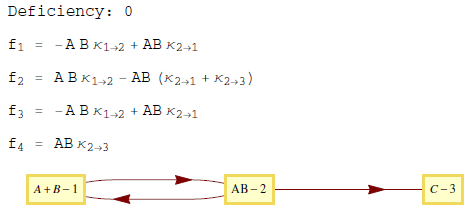
reaction-networks.m — a Mathematica package with a custom function MakeCRN. This function takes as input a description of a chemical reaction network and returns as output (1) the deficiency of the network, in the sense of Chemical Reaction Network Theory (CRNT); (2) the polynomial equations arising from mass-action kinetics; and (3) the directed graph on the CRNT "complexes". For more information on CRNT, see Gunawardena, "Chemical Reaction Network Theory for in-silico biologists", preprint, 2003.
- developers: Robert Karp, Tathagata Dasgupta, Joseph Dexter
- citations: Karp, Perez Millan, Dasgupta, Dickenstein, Gunawardena, J Theor Biol, 2012; Dexter, Dasgupta, Gunawardena, submitted, 2014.
- requires: Mathematica 9.
- usage: after loading the package into Mathematica, a chemical reaction network is specified as an input by giving a list of reactions, with each reaction described as a pair consisting of a source "complex", or sum of source components, and a product "complex", or sum of product components. If a third element, r, is added to the pair, the reaction is treated as reversible. In the output polynomials, the rate constants are indexed according to the numbering of the complexes in the graph. For example,
| | |
MakeCRN[{{A + B, AB, r}, {AB, C}}] | |  |
.
- Further examples can be found in the Mathematica notebook which is provided as supplementary information to Dexter, Dasgupta, Gunawardena, submitted, 2014.
linear framework
The linear framework provides a method for time-scale separation in biochemical systems (Gunawardena, PLoS ONE, 2012; Mirzaev, Gunawardena, Bull Math Biol, 2013). It is based on a labelled, directed graph on which a linear (Laplacian) dynamics is defined. If the graph is strongly connected, the steady state of the dynamics is given by the Matrix-Tree Theorem in terms of the rooted, spanning trees of the graph.
MTT.py — a python script which computes the rooted, spanning trees of a graph using Uno's algorithm (Takeaki Uno, "An algorithm for enumerating all directed spanning trees in a directed graph", Springer LNCS 1178, 1996; PDF).
- developer: Felix Wong
- citation: Ahsendorf, Wong, Eils, Gunawardena, "A framework for modelling gene regulation which accommodates non-equilibrium mechanisms", submitted, 2014.
- requires: Python 2.7 or later.
- usage: python MTT.py graph-name.txt
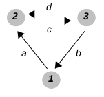
- graph-name.txt should be a text file containing a description of the graph as a list of triples (i,a,j), denoting an edge from vertex i to vertex j with label a:
| example graph | | example.txt file |
 | |
# 23 October 2013
# example graph description

(1,a,2) (3,b,1) (2,c,3) (3,d,2)
|
- for each vertex i in the graph, the script writes an output file, graph-name-i.txt, listing the spanning trees rooted at i:
| example-1.txt | | example-2.txt | | example-3.txt | |
0 1 1 0
| |
1	1	0	0
1	0	0	1
| |
1 0 1 0
| |
Each spanning tree is encoded as a binary string, indicating which edges are present, following the edge ordering in example.txt. The script also writes a condensed version of the input file, called example-parsed.txt, which can be more easily read by the Mathematica notebook described next.
graph-interface.nb — a Mathematica notebook for constructing and manipulating the polynomials that come from the Matrix-Tree Theorem.
- developer: Felix Wong
- citation: Ahsendorf, Wong, Eils, Gunawardena, "A framework for modelling gene regulation which accommodates non-equilibrium mechanisms", submitted, 2014.
- requires: Mathematica 8 or later.
- usage: set GraphName to the name of the graph description file: GraphName = "example", if the file is example.txt. MTT.py should have been run previously to generate the example-i.txt and example-parsed.txt files and these files should be in the same directory as the notebook. Execute the Mathematica functions in the notebook as required.
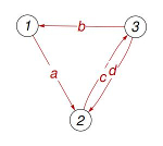
- The notebook can display the graph as a consistency check and it can calculate the components of the vector ρ, which is the basis vector for the kernel of the Laplacian (for a strongly-connected graph), considered as a polynomial function of the labels in graph-example.txt.
 |
|
rho1[a,b,c,d]= bc
rho2[a,b,c,d]= ab + ad
rho3[a,b,c,d]= ac
|
These expressions can be interrogated using built-in Mathematica functions for manipulating polynomials and can be used for various steady-state calculations, depending on the biological context.
Examples
- From the paper Ahsendorf, Wong, Eils, Gunawardena, submitted, 2014.
- kimoshea.txt (graph description file) and kimoshea.tar.gz (gzipped archive containing all files and programs). This is the PHO5 gene regulation example in Figure 7 of the paper, which is taken from Kim, O'Shea, "A quantitative model of transcription factor-activated gene expression", Nat Struct Mol Biol 15:1192-8 2008, PMID. The gene regulation function is given in full in the accompanying Additional File.
- kimoshea-fits.tar.gz (gzipped archive containing a Mathematica notebook and accompanying files). This suite of programs undertakes the fit of the calculated gene regulation functions to the experimental data for PHO5 promoter variants, as shown in Figure 8 of the paper.
- product.txt (graph description file) and product.tar.gz (gzipped archive containing all files and programs). This is the example of the product graph in Figure 9 of the paper, which is analysed further in the accompanying Additional File.
